XO

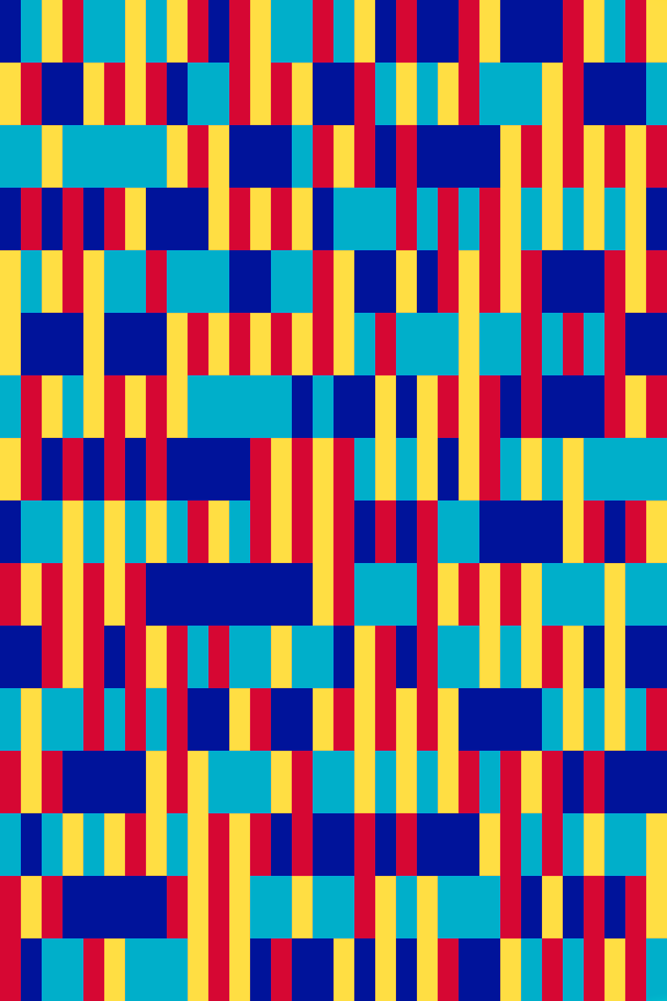
Almost a year after I ran out of ideas for my color grids, a new idea came to me, and this is the result: 

This grid was generated following a similar rule set to the featured grid in Solving a Hard Problem (SaHP).  Likewise, the grid has 16 rows and 32 columns, with each cell being 3 times as tall as it is wide.  

It follows the same adjacency restrictions, and like the SaHP grid, the four colors are evenly distributed in each row and column: 

 

 

It does not however follow either the 3rd (each 4×4 block) or 4th (central rectangle) distribution sets of the SaHP grid.  

There is one other distribution set – and it is the reason for the “XO” name.  Can you figure out why? To avoid spoiling the problem for those who want to solve it, here are 141 periods:

…

…

…

…

…

…

…

…

…

…

…

…

…

…

…

…

…

…

…

…

…

…

…

…

…

…

…

…

…

…

…

…

…

…

…

…

…

…

…

…

…

…

…

…

…

…

…

…

…

…

The answer of course has something to do with the black border that divides the grid into sixteenths.  In fact, the original image I chose to feature on this page did not have the border.  I created the image with the border to help explain the distribution set that is the reason for it’s name, and I liked it enough to use it as the main image.  Here it is without the border:

The Uneven Distribution Set

The colors are evenly distributed in each quadrant of the grid.  This is a consequence of the 3rd distribution set, which determines how many of each color are in each sub quadrant, which are separated by the black borders.  

The colors for the 32 cells in each sub quadrant are distributed in one of the two following ways:  12 of 1 color, 8 of 1 color, and 6 of 2 colors, OR 10 of 2 colors, 8 of 1 color, and 4 of 1 color.  

Each quadrant has a featured color – with 12 of that color in two of the sub quadrants, and 4 of that color in the other two.  The featured color is paired with another color (red is paired with gold and vice versa, and the blues are paired with each other) – the paired color fills 8 cells in sub quadrant.  The other two colors fill 6 cells in two quadrants and 10 cells in the other two.  

Turquoise is featured in the top left quadrant, gold in the top right, red in the bottom left and dark blue in the bottom right:

The following shows the exact counts of each color in each sub quadrant:

The X and O 

The sub quadrants where the quadrant’s featured color fills 12 cells form an X, with the other sub quadrants forming an O: 

The “X” can be seen without the special highlighting in my opinion, particularly the red/gold forward slash.  The “O” is a bit more subtle:

Here is one more  visualization based on the sub quadrants:

How and Why

My original idea when I decided to resume this project to try out uneven distribution sets was much simpler:  for each quadrant, one color would fill more cells than the other 3 colors, which would fill the same amount of cells (my initial plan was a 44/28/28/28 distribution).  Like the featured grid, each color would be featured in one of the quadrants.  I even coded this into my program and set it to work using the same rule set as SaHP but replacing the 4×4 block distribution set with this one.  Shortly after it started, I realized the flaw with my plan:  the uneven distribution set made the even row and column distribution sets impossible to satisfy.  For example, suppose red is featured in the top left quadrant, and fills 44 of the 128 cells.  It will also fill 28 cells in the top right quadrant, where another color is featured.  Thus it will fill 72 of the 256 cells in the first 8 rows, instead of the 64 cells it needs to fill to satisfy the row distribution set.  

Disappointed that my plan wouldn’t work but not ready to give up on the idea, I decided to keep the colors evenly distributed in each quadrant, with the uneven distribution set dictating the colors in the sub quadrants.  Thinking ahead, I came up with the “X” idea not for visual reasons, but because it was necessary for the central rectangle distribution set from SaHP to work.  

The first distribution I tested was different than the featured grid:  the featured color would fill 11 cells in the X sub quadrants and 5 cells in the O’s, while the other 3 colors would fill 7 and 9 cells respectively.  Although the X was designed to make the central rectangle set possible, I first tried it out without this set as I knew it would take my program far less time (I also felt that because the “X” points towards the center, the central rectangle set wasn’t necessary, as it’s main purpose was to add a bit of a central focus to the grids with only even distribution sets).  

I was really happy with the results (#1  below), and planned to use the first grid my program generated following these rules for this page, with the title, “Odd” based on the fact that I could summarize the uneven distribution set with the following:  1 color fills either 5 or 11 cells, while 3 colors fill either 7 or 9 cells (an alternate title was “day job at 7-11, based on the fact that the sub quadrants had either a 7/11 or a 9/5 split).  I also tried it with the central rectangle set, which took 2 days for my program to solve compared to just 2 hours.  In terms of difficulty, this rule set is even harder than SaHP set, but unfortunately I was disappointed with the results (#2 below) and preferred the easier rule set visually.  

The only problem I had with the grid I planned to feature on this page was that it looked slightly imbalanced because red and gold were featured in the right two quadrants with the blues featured in the left quadrants.  The program was randomly choosing the featured color for each quadrant – to address this I told it to feature red/gold and dark blue/turquoise in opposite quadrants and my program produced grids both with and without the central rectangle set.  While I liked the results, it added to my confusion in terms of writing this page, as I couldn’t decide between the 4 grids (1 of which is #3 below)  I generated without the central rectangle set and the 1 (#4 below) I generated with it (which I liked much better than the previous one).  

A week after sitting on it, the 12-8-6-6/4-8-10-10 idea popped into my head, with the 8 color being the complementary color to the 12/4 color, though to be honest I wasn’t expecting much of a difference.  I was pleasantly surprised, and the featured grid is the first of two grids generated following this distribution.  As I write this, my program is going on day 3 of working on the same rule set with the central rectangle set which it will eventually solve, though I don’t expect the results to be better visually than this grid. 

This distribution is just a bit more extreme/unbalanced compared to the original 7-11/9-5 distribution.  Since I liked the results, I took it one step further and tried a 13-9-5-5/3-7-11-11 split.  While the results were interesting (#5 below) and I thought about using one of the grids generated with the new split, I ultimately felt that these grids crossed the threshold where the results are obviously not random and decided to stick with the featured grid.  

Below are grids following each of the rule sets mentioned along with the featured grid:

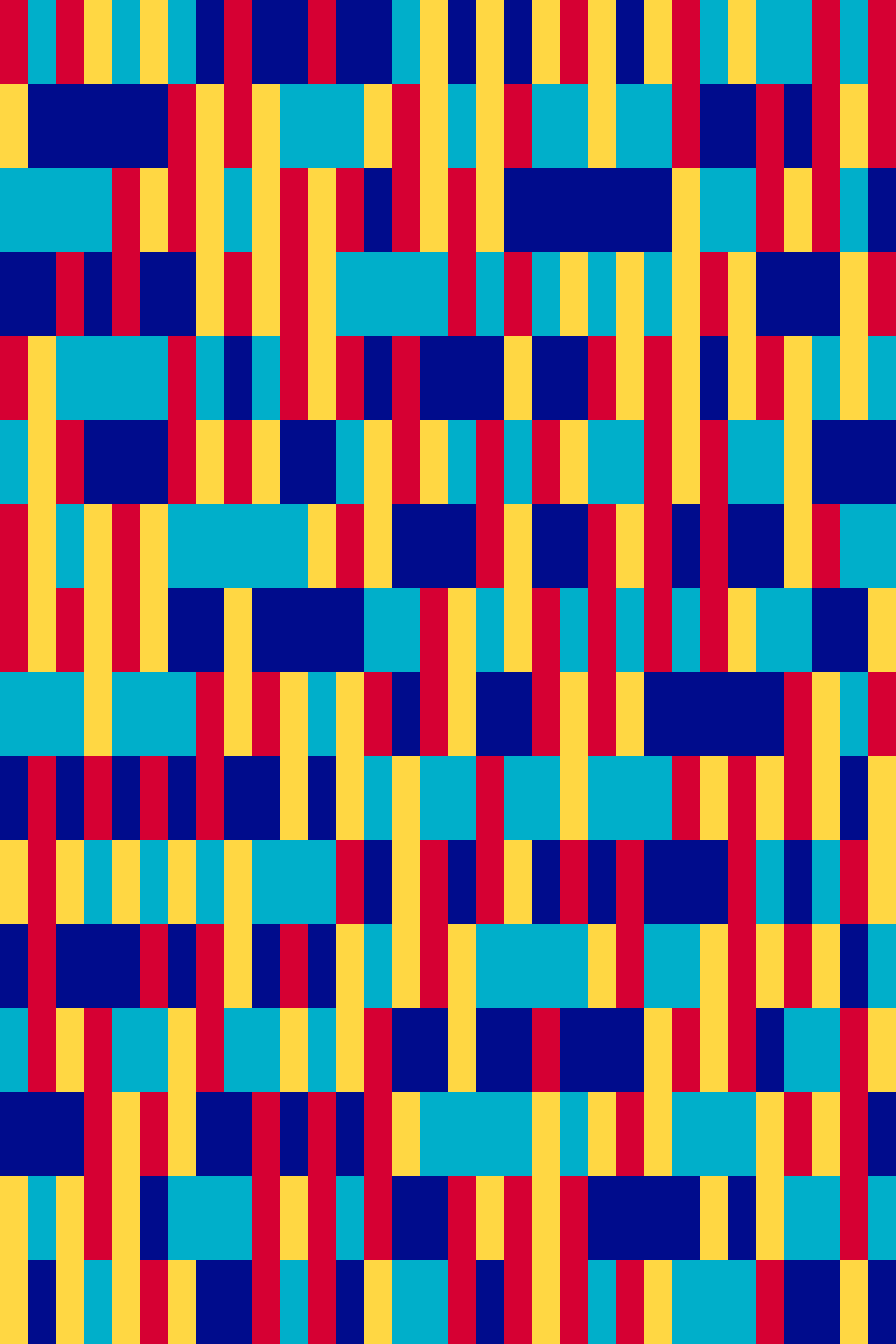
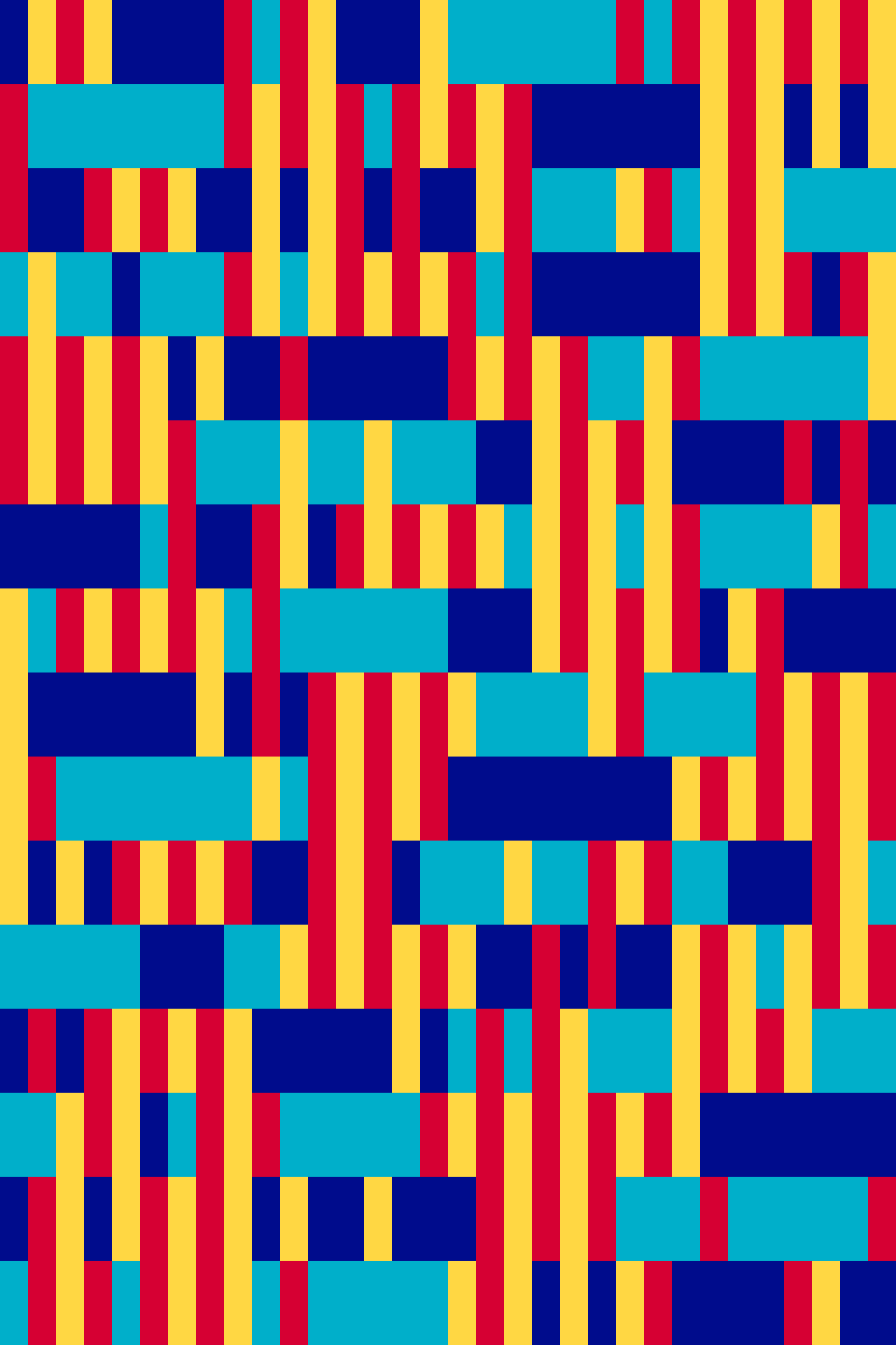
Here is a table:

Grid	Feat Col	X Dist	O Dist	CR
#1	T/G/R/DB	11-7-7-7	5-9-9-9	No
#2	T/DB/R/G	11-7-7-7	5-9-9-9	Yes
#3	T/G/DB/R	11-7-7-7	5-9-9-9	No
#4	DB/R/T/G	11-7-7-7	5-9-9-9	Yes
#5	T/G/DB/R	13-9-5-5	3-7-11-11	No
#6	T/G/DB/R	12-8-6-6	4-8-10-10	No

Feat Col = featured color in each quadrant, starting with the top left and going clockwise.  

CR = with or without the central rectangle distribution set (see Solving a Hard Problem).