Filtering Levels Using a Formula
Steps:
- Generate the Levels
- Collect the Data
- Evaluate Levels
- Generate a Formula
- Pick the Levels using the Formula
Generate Levels and Collect the Data
Levels are generated using my level generator for each board design in the pack. As the levels are generated – statistics are calculated and stored in a database about each level. This includes:
- # of Dots
- # of Portals
- # of Bridges
- # of Portals Crosses
- # of “Filler” Lines (Lines <=4 tiles that don’t cross a portal)
- # of Lines crossing portals
- # of Lines crossing multiple portals
- Maximum portals crossed by a single line
Evaluate Levels
My test version of CTD: Shadows and CTD Portals allows me to give each level a rating from 1-10 after completing the level.
I did this for thousands of levels – mostly in CTD: Shadows.
Generate a Formula
I used the statistics about each level and the ratings and ran a linear regression analysis to generate a formula that calculates the expected rating of a level based on its statistics.
Pick the Levels Using the Formula
The above formula is then used to filter the generated levels to a specific percentage – the percentage is based on how similar the top rated levels look. If I only picked the top levels, there would be a lot less variety in the games.
The Filtering Problem
Scenario:
- 1000 levels were generated for a board design – but I only need 10 for the game
This scenario is common – my level generator is pretty fast. I have a database with over 10 million levels generated by the program – yet there are only 3,500 in CTD: Shadows and CTD: Portals combined.
Q: Why not pick the top 10 rated levels?
A. The levels will look too similar to each other.
Q: So, how can I use the formula?
A: I can tell my program to find the top X% of the levels – and then have it randomly pick 10 levels from that group.
Q: What is X?
X is a number that I choose for each board design. The number has to be sufficiently high that there will be enough variety (by my subjective opinion) in the set of levels chosen.
Q: How do I pick X?
Generally, the more complex the board design the lower the X I assign it. I judge complexity based on the size of the board, the pattern of the walls, and number of portals.
I used a range of about 3 to 70% for X in CTD: Shadows/Portals.
Wasted Levels
Let’s suppose I pick an X of 10% for the above scenario. That means my program will pick 10 random levels from the top 100 levels.
But, if I only made 100 levels – it would still pick the top 10% of those levels and the results would be similar.
Q: Why did I make 1000 levels then?
A: Because it didn’t take much time to make them. Also – I will generally tell the program to include the top rated level with the set. The top rated level will generally be “better” if I make 1000 levels vs. 100.
An Alternative Approach – Similarity Filtering
I created the formula mainly while testing levels for CTD: Shadows. The formula doesn’t apply as well with CTD: Portals – though I used it anyway. It also is pretty terrible for the basic levels in Connect Unlimited.
In CTD: Portals – I found that I didn’t like the top rated levels that were included with the random X%. Effectively this made generating extra levels a complete waste of computer time and database space.
I also found that I valued uniqueness above all else when selecting my favorite levels.
So – I developed a method to try to find the unique levels.
What Makes a Level Unique?
Criteria:
- The level doesn’t look like most other levels.
- There isn’t another level that looks too much like the level.
- It has unique characteristics that stand out from other levels.
Similarity Maps Address Criteria #1
Read about similarity maps and how they are generated here: Similarity Maps
Here’s one of the maps:

This level was compared against 29 other levels of the same size. The shading is based on the average similarity of each tile for each comparison.
The average opacity of the shading for the map is the levels average similarity score. This map scores 59%.
…. but not Criteria #2 and 3
On the Similarity Maps page I stated that the similarity map is the new formula for selecting levels. This was a bit of an exaggeration (ok, lie). While the average similarity score is the most important factor in the similarity filtering – there are two other components that are meant to address criteria #2 and #3:
The Highest Similarity Score For a Level Addresses #2
Criteria 2: There isn’t another level that looks too much like the level.
The following shows the level that had the highest similarity score (among the 29 comparisons made):

The levels have a similarity score of 75%.
Showing Both in One Image
I can average the shading from the above comparison with the original similarity map:

Filtering with Similarity Maps (and a bit more)
Read: Similarity Maps to see how the maps are generated and levels are scored.
On that page I stated that the maps alone are the filtering formula – this is a bit of an exaggeration (OK, lie).
The maps address the first criteria but only the first criteria. It ends up being weighted the highest of any other component – and the two other components are based on the same process, but not the map itself.
Criteria 2: There isn’t another level that looks too much like the level
An issue with using the maps alone is that there could be two identical levels in the set of levels used to generate the maps that still score “well” by the map.
To address this, when comparing a set of levels the highest similarity score for each level is stored and used in the formula.
Criteria 3: The level has unique characteristics that stand out from other levels
This is sort of addressed with the first two criteria (in fact, all the scores are very highly correlated with each other), but for good measure I also calculate a line uniqueness score for each level.
The line uniqueness score is calculated with a similar process to the similarity score – except that each line is compared against every other line in every other level (and every rotation), to find the line that consumes the most tiles. The tiles that remain for each line are counted and divided by the total number of tiles for the score.
Unlike similarity scores, a higher uniqueness score is better.
All in One Formula
The final formula for similarity filtering is as follows:
A * Average Similarity Score (the similarity map) plus
B * Max Similarity Score minus
C * Uniqueness Score.
A, B, and C vary depending on the set of levels and the stage of the filtering.
Adjusting for Line Length
The formula above works pretty well on its own – but there is a tendency to over value levels with a couple of long, crazy lines and many short “filler” lines.
To adjust for this:
The consumed tiles are counted for each line, and the count of the remaining tiles are divided by the total cells in the line.
This percentage is multiplied by the square root of the total tiles in the line.
These values are summed for each level, and then divided by the sum of the square roots of the line lengths.
Note that only consumed (red or magenta in the map) tiles are counted in this formula – it doesn’t care about the tiles that a line consumes itself.
This adjustment effectively penalizes both short and long lines:
- Short lines are counted more in the formula than before. In the similarity maps, these lines tend to have a lot of red and very little blue.
- Long lines are counted less in the formula – these lines are usually very blue with (relatively) little red.
Where’s the Blue?
The blue tiles are counted indirectly by summing the red tiles in the other level (and adjusting for line length, as described). Magenta tiles end up being counted twice as a result.
When comparing two levels, the similarity score is always the same for both levels no matter what the distribution of red and blue tiles are in the map.
Filtering Large Sets of Levels
Individual Comparisons Involve a lot of Calculation
Consider two square levels that are 10×10 with 10 lines each that are 10 tiles long
To calculate the similarity score – each line is compared against every other line to find the number of tiles that intersect.
If not for hash sets – an individual line comparison would have to compare each tile in the first line against every other tile in the second line.
Hash sets make the individual line comparison much faster – but there are still 10×10 = 100 line comparisons to make. Not to mention that to account for rotation – 4 times as many comparisons are made.
The Time to Calculate Comparisons For a Set of Levels Increases Exponentially with the Size of the Set
Comparing 10 levels against each other requires 9+8+7+6+5+4+3+2 + 1 = 45 comparisons, while 20 levels requires 19+18 + 17 + 16…+1 = 190 comparisons. The uniqueness calculation requires for 10 levels requires an additional 9*10 = 90 comparisons for 10 levels and 19*20 = 380 comparisons.
Splitting A Set of Levels Into Small Groups
Comparing a set of 1000 levels against each other would require 499,500 + 999,000 = 1,498,500 comparisons.
If instead we split the 1000 levels into 100 groups of 10 levels and compare each group against each other, there are only (45 + 90) * 100 = 13,500 comparisons to be made.
Accounting For Luck
A levels similarity score depends on the levels that it is being compared against. Thus, if we split 1000 levels into 100 random groups of 10 levels, some levels will score higher than they should and some will score lower based on luck alone.
There are three ways this is dealt with:
- The levels are split into random groups multiple times (usually two) per each pass, and the score for each level is the average of the two scores.
- Levels are filtered based on scores in multiple iterations. Typically, each iteration filters out half of the levels. The process is then run again on the remaining levels, until the desired number of levels is reach. For example:
- Start with 1000 levels with the goal of picking the top 10 levels.
- After iteration 1, 500 levels remain
- After iteration 2, 250 remain
- After iteration 3, 125 remain, and so on until only 10 levels remain
- Scores from previous iterations are kept for future iterations. After the scores are calculated for an iteration, each level is assigned a total weighted score with the most recent scores counted more.
One vs. Two-Way Comparison
My first approach towards filtering levels based on similarity used a one-way comparison for each level.
This counted only the red/magenta tiles for each level – and didn’t care about the blue tiles.
The resulting scores were not symmetrical – typically, the level with fewer dots and longer lines would score higher than its counterpart.
Consequently, levels with longer lines and fewer dots were favored each iteration.
This didn’t bother me as much as it should have – since my formula liked these levels.
The problem was – this method of filtering didn’t solve the filtering problem, even by its own measure of success.
The following chart shows what happened with this method:

Wt Avg – The weighted average sim score of the entire set after X iterations. More recent scores are weighted higher
Last Avg – The average sim score of the entire set for the Xth iteration. These 2 numbers are always the same on the 1st iteration (because there are no other scores to consider in the weighted average).
Top W Avg – The weighted average sim score of the top 50% of levels remaining after X iterations. These are the levels that move on to the next iteration.
Top L Avg – The average sim score of the top 50% of levels (by weighted average) for the Xth iteration.
You don’t have to pay attention to the numbers – just notice that the lines are flat. Basically – the similarity scores barely improved from the 1st iteration to the last iteration (and almost all the improvement is accounted for in the 1st iteration).
The reason: the levels selected for each iteration usually score worse the next iteration. I call these levels greedy.
Switching to Two-Way Comparison
Counting the blue tiles makes each levels score symmetrical when compared against another level.
Using this method of scoring – the levels that advance each iteration usually score better the next iteration.
Here’s the chart:

Filtering by Uniqueness Has No Limit
Average maps after 0 through 7 iterations of similarity filtering.


The Filtering Problem Shown with Similarity Maps
I’ll use a much simplified version of the formula I used to rate levels to show an example.
I’ll base the formula completely on the number of dots. For one set, I’ll pick levels with the least number of dots, and the 2nd set, I’ll pick levels with the most number of dots. Here are the maps:
Few Dots, Long Lines


Lots of Dots, Short Lines


Neither set looks particularly appealing – and you can see how the levels look quite similar. The 2nd set doesn’t get a “bad” similarity score – just bad levels.
Perfectly Imperfect
The Level Generator is the heart of the program – essential for all Connect the Dots games and the computer generated artwork.
If the program didn’t make good levels – both from a game play and aesthetic perspective, neither the games or the art would be any good.
It was relatively easy making a program generate levels for a basic square board. Connect the Dots: Shadows has about 200 different board designs – all with multiple sectors, and tons of different wall patterns.
This required a ton of additional work for the level generator – at least to make the levels look natural.
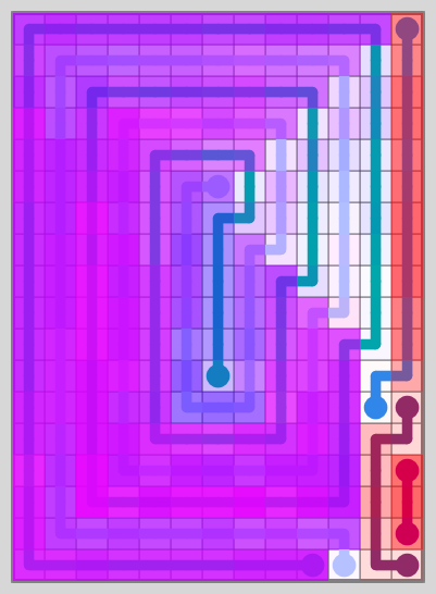
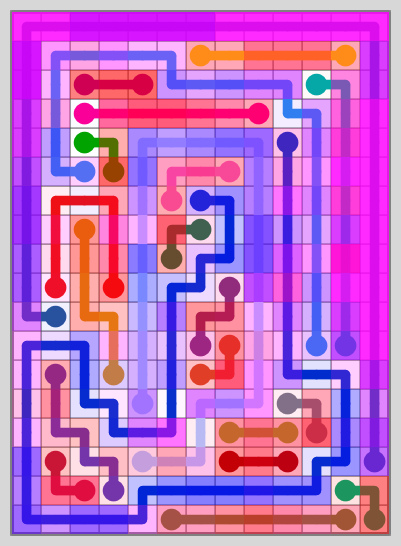
Here is an example:

This level has intricate walls – yet there are just 6 lines covering a total of 247 squares. The lines follow the walls.